Prophet vs XGBoost is a common question when you forecast demand that depends on the weather: calls to a help desk, deliveries, or cars that won’t start on a frosty morning. Prophet gives you trend, seasonality, holidays and linear regressors in a few lines. XGBoost gives you a flexible model over whatever features you build. I wanted to see how they compare for demand forecasting with weather regressors, so I built a synthetic daily series of service calls with known weather effects and backtested both, honestly, including the part most tutorials skip: at prediction time you don’t know tomorrow’s weather, only a forecast of it.
The question came from the AI Native Netherlands meetup at Elastic in Amsterdam on 15 January 2026. ANWB, the Dutch motoring club, opened with “How AI is helping you back on the road”. One slide named XGBoost + Prophet to predict number of car trouble cases. Another, “People ← Trust → Model”, put a planner’s spreadsheet next to the model. The spreadsheet took last week’s cases per day and added 250 when the temperature dropped below 5 and another 250 when precipitation was above 0.5. The model took day, temperature, precipitation and yesterday’s count. That slide is all I know about their setup. Everything below is my own experiment on made-up data, not how ANWB built theirs.

The “People ← Trust → Model” slide from the ANWB talk.
Versions. Python 3.12.13 on macOS 26.6 (Apple M1 Pro), prophet 1.4.0 with the cmdstanpy 1.3.0 backend, xgboost 3.4.1, pandas 3.0.6, numpy 2.5.3, holidays 0.105 and matplotlib 3.11.2. I checked the APIs against the Prophet docs on holidays and regressors, diagnostics and uncertainty intervals, the XGBoost parameter reference and its scikit-learn estimator guide, and the installed docstrings.
All numbers in this post come from synthetic data. They show how the methods behave when you know the truth. They are not a benchmark of either library on real demand.
A synthetic series with known weather effects
Five years of daily calls, 2021 to 2025. I know every driver because I wrote them:
import numpy as np, pandas as pd, holidays

rng = np.random.default_rng(42)
dates = pd.date_range("2021-01-01", "2025-12-31", freq="D")
doy = dates.dayofyear.to_numpy()

# Weather: seasonal temperature + AR(1) anomalies; wet days with gamma amounts (mm)
clim = 10.5 - 7.5 * np.cos(2 * np.pi * (doy - 15) / 365.25)
anom = np.zeros(len(dates))
for i in range(1, len(dates)):
    anom[i] = 0.8 * anom[i - 1] + rng.normal(0, 1.8)
temp = (clim + anom).round(1)
p_wet = 0.50 + 0.12 * np.cos(2 * np.pi * (doy - 320) / 365.25)
precip = np.where(rng.random(len(dates)) < p_wet, rng.gamma(0.8, 4.0, len(dates)), 0.0).round(1)

# Demand
t = np.arange(len(dates)) / 365.25
base = 1000 * (1 + 0.03 * t)                                            # +3% a year
weekly = np.array([1.10, 1.02, 1.00, 1.00, 1.06, 0.88, 0.80])[dates.dayofweek]  # Mon..Sun
summer = 1 + 0.08 * np.exp(-0.5 * ((doy - 210) / 18) ** 2)              # late-July travel peak
nl = holidays.NL(years=range(2021, 2026))
hol = np.where([d in nl for d in dates.date], 0.75, 1.0)                # public holidays -25%

cold = 35 * np.clip(3 - temp, 0, None) ** 1.3        # batteries die below about 3 C
heat = 15 * np.clip(temp - 20, 0, None)              # hot days
rain = 60 * np.log1p(precip)                         # wet roads, diminishing returns
black_ice = np.where((temp < 1) & (precip > 0.5), 120, 0)

mu = base * weekly * summer * hol + cold + heat + rain + black_ice
calls = rng.negative_binomial(150, 150 / (150 + mu))  # over-dispersed counts
The full script wraps this in a function and returns a DataFrame with ds, y, temp, precip and is_holiday, so the same seed gives the same series every run. The mean is about 1,108 calls a day. The weather effects are deliberately non-linear: nothing happens until it gets cold, then it ramps up, and frost plus rain adds a bump. The negative binomial noise alone has a standard deviation of about 96 calls a day around 1,100, so no model can get much below a mean absolute error (MAE) of about 75 to 80.
Prophet with holidays and weather regressors
Prophet wants a ds and y column. Country holidays and extra regressors are one call each:
from prophet import Prophet

def make_prophet(regs):
    m = Prophet(weekly_seasonality=True, yearly_seasonality=True,
                daily_seasonality=False, interval_width=0.8)
    m.add_country_holidays(country_name="NL")
    for r in regs:
        m.add_regressor(r)
    return m

m = make_prophet(["temp", "precip"]).fit(df[["ds", "y", "temp", "precip"]])
fc = m.predict(future[["ds", "temp", "precip"]])
fig = m.plot_components(fc)
add_country_holidays uses the holidays package. m.train_holiday_names lists what it found for the Netherlands: New Year’s Day, Easter, King’s Day, Ascension Day, Pentecost, Christmas and so on. add_regressor standardises the column by default (unless it is binary) and adds a linear, additive term. The docs are explicit that “the extra regressor must be known for both the history and for future dates”. Remember that sentence.
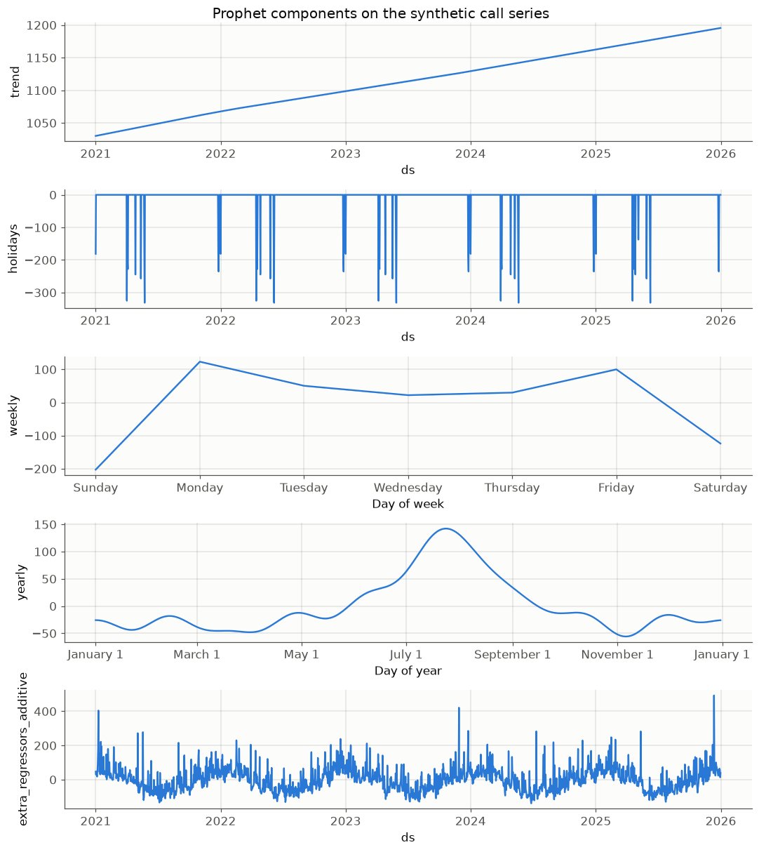
Prophet’s components on the full synthetic series: trend, holidays, weekly, yearly and the weather regressors.
The components plot recovered what I put in: a rising trend, holiday dips, low weekends, a late-July bump. prophet.utilities.regressor_coefficients(m) gave −8.3 calls per °C and +15.7 calls per mm. Those are linear averages of effects that aren’t linear: the real temperature effect is zero above 3 °C and steep below it. The weather component also shows a yearly wave, because temperature is seasonal and competes with the yearly seasonality term.
The fix is feature engineering, not a different library. I added a second Prophet variant with cold = max(0, 5 − temp) (degrees below 5 °C, the threshold from the spreadsheet rule) and log_precip = log1p(precip) as regressors.
XGBoost with lags, rolling windows, calendar and weather
XGBoost knows nothing about time, so you hand it features. The horizon decides which lags you may use. I forecast 7 days ahead, as for next week’s roster, so every lag is at least 7 days old. “Yesterday’s count” is only available if you forecast one day ahead (or forecast recursively).
import xgboost as xgb

def add_features(d):
    d = d.copy()
    for lag in (7, 14, 21, 28, 364):
        d[f"lag_{lag}"] = d.y.shift(lag)
    d["roll7_mean"] = d.y.shift(7).rolling(7).mean()
    d["roll28_mean"] = d.y.shift(7).rolling(28).mean()
    d["roll28_std"] = d.y.shift(7).rolling(28).std()
    d["dow"], d["doy"], d["month"] = d.ds.dt.dayofweek, d.ds.dt.dayofyear, d.ds.dt.month
    return d

CAL = ["lag_7", "lag_14", "lag_21", "lag_28", "lag_364", "roll7_mean", "roll28_mean",
       "roll28_std", "dow", "doy", "month", "is_holiday"]
WX = ["temp", "precip"]

XGB_PARAMS = dict(n_estimators=600, learning_rate=0.03, max_depth=5, subsample=0.8,
                  colsample_bytree=0.8, min_child_weight=3, tree_method="hist")
model = xgb.XGBRegressor(**XGB_PARAMS)
model.fit(train[CAL + WX], train.y)
shift(7) before rolling matters: a rolling mean that includes the last six days would leak information you won’t have a week ahead. I used fixed hyperparameters and no tuning. If you tune, pass early_stopping_rounds to the constructor and an eval_set that comes after the training data in time. The scikit-learn guide notes that XGBoost doesn’t split data for you, and that predict then uses the best iteration automatically.
A backtest that respects time
Random k-fold cross-validation is wrong for time series: it trains on the future. Use rolling-origin evaluation instead. Prophet has it built in:
from prophet.diagnostics import cross_validation, performance_metrics

cv = cross_validation(m, initial="1095 days", period="5 days", horizon="7 days")
performance_metrics(cv, rolling_window=1)   # one row over all forecasts
That trains on the first three years, then makes a forecast every 5 days through 2024 and 2025: 145 cutoffs, 1,015 forecast days, 23 seconds on my laptop. I used a 5-day period so cutoffs don’t always fall on the same weekday. With a 7-day period, lead day 1 would always be the same day of the week.
XGBoost has no equivalent, so I wrote an expanding-window loop over the same cutoffs (taken from cv.cutoff.unique()), training only on rows with ds <= cutoff. I refitted Prophet in the same loop as well, because I needed to swap the future weather (next section). My manual Prophet MAE was 93.7 against 93.6 from cross_validation, so the loops agree. The whole loop, four Prophet fits and four XGBoost fits per cutoff, took about 10 minutes.
Metrics: MAE, MAPE and WAPE
- MAE is in calls per day, which is what a planner understands.
- MAPE averages the percentage error per day. It explodes near zero, can’t be computed on days with no demand, and weights a quiet holiday as much as a frosty Monday. Here volumes never get near zero, so it is close to WAPE. On the 33 holiday days, though, Prophet’s MAPE was 11.2% against 8.1% overall.
- WAPE is the sum of absolute errors divided by total demand: “what share of the calls did we misplan”. It’s the one I’d report to the business.
- Bias (mean of forecast minus actual) tells you which way you’re wrong, which matters more for staffing than a few points of MAE.
Results: Prophet vs XGBoost, with and without real weather
First the comfortable version, where the backtest feeds each model the actual weather for the next 7 days, which is what cross_validation does with regressors:
| Model (actual weather) | MAE | MAPE | WAPE | Bias |
|---|---|---|---|---|
| Same day last week | 150.2 | 13.2% | 13.0% | +1.3 |
| Spreadsheet-style rule | 149.3 | 13.2% | 12.9% | +23.1 |
| Prophet, no weather | 101.4 | 8.8% | 8.8% | −4.2 |
| Prophet, temp + precip | 93.7 | 8.1% | 8.1% | −2.9 |
| Prophet, engineered weather | 81.3 | 7.1% | 7.0% | −1.5 |
| XGBoost, no weather | 111.4 | 9.5% | 9.6% | −20.5 |
| XGBoost, temp + precip | 88.8 | 7.6% | 7.7% | −28.3 |
| Ensemble (Prophet raw + XGBoost) | 86.6 | 7.5% | 7.5% | −15.6 |
The “rule” is my version of the shape on the ANWB slide: last week’s value plus a bump below 5 °C and another above 0.5 mm, with the bumps fitted by least squares on the training data. It barely beat the naive forecast. The fitted cold bump was only about 8 calls, because last week was usually cold too, so last week’s count already contained most of the effect. A rule like that is easy to trust and hard to improve by hand. That is why the slide put people, trust and the model on the same line.
With raw weather, XGBoost beat Prophet (88.8 against 93.7) because trees learn the cold threshold on their own. Give Prophet the right features and it won (81.3). The simple average of Prophet and XGBoost beat both of its members. XGBoost ran consistently low, by 28 calls a day on average and by 71 on days below 3 °C: trees can’t predict beyond the range they’ve seen, and a cold snap or a growing trend sits at the edge of that range.
The weather-forecast pitfall
In production you have a weather forecast for next week, not the weather. A backtest with actual weather in the future rows quietly assumes a perfect forecast. To measure the gap I made “forecast” weather from the actual weather plus an error that grows with lead time:
def forecast_weather(frame, lead, rng):
    out = frame[["temp", "precip"]].copy()
    out["temp"] = frame.temp + rng.normal(0, 0.8 + 0.35 * lead)          # degrees C
    wet = frame.precip > 0
    flip = rng.random(len(frame)) < (0.08 + 0.03 * lead)                 # wrong wet/dry call
    amount = frame.precip * rng.lognormal(0, 0.3 + 0.1 * lead)           # wrong amount
    new_wet = np.where(flip, ~wet, wet)
    out["precip"] = np.where(new_wet, np.where(wet, amount, rng.gamma(0.8, 4.0, len(frame))), 0.0)
    return out
These error sizes are my assumption, not a measured property of any weather service. I fitted the models exactly as before and only swapped the future weather columns at prediction time.
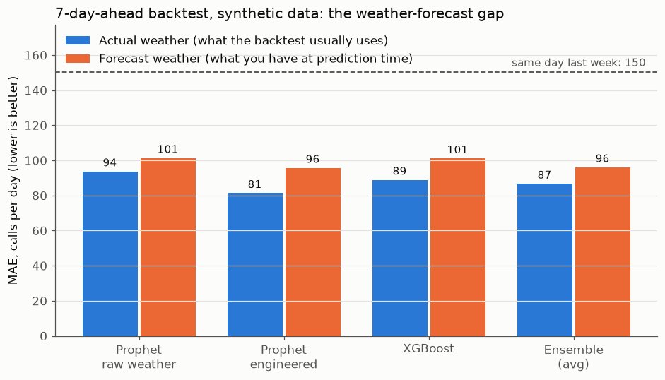
7-day-ahead MAE on the synthetic series, actual weather vs noisy forecast weather. The ensemble here averages Prophet with raw weather and XGBoost.
| Model (forecast weather) | MAE | WAPE | Change vs actual weather |
|---|---|---|---|
| Prophet, temp + precip | 101.3 | 8.8% | +8% |
| Prophet, engineered weather | 95.6 | 8.3% | +18% |
| XGBoost, temp + precip | 101.0 | 8.7% | +14% |
| Ensemble (Prophet engineered + XGBoost) | 95.7 | 8.3% | — |
Prophet 1.4 regressor_predictor (no external forecast) | 100.3 | 8.7% | — |
Three things stood out:
- The best model lost the most. The engineered Prophet model went from 81.3 to 95.6. A hinge at 5 °C is sensitive exactly where forecast errors flip a day across the threshold. On days below 3 °C its MAE went from 95 to 128.
- Weather still paid off, a little. With forecast weather, Prophet improved on its no-weather version by 6% (95.6 against 101.4) and XGBoost by 9% (101.0 against 111.4). That’s much less than the actual-weather backtest promised.
- Training on archived forecasts didn’t help here. I retrained XGBoost on historical rows with simulated forecast weather instead of actuals, which is the usual advice. MAE stayed at 101.5. My errors are independent noise with no systematic bias, so the model just learned weaker weather effects. With real archived forecasts, which have systematic biases a model can learn, it’s still worth testing.
Prophet 1.4.0 added regressor_predictor to add_regressor, which fits a nested Prophet model to forecast the regressor itself. For weather that amounts to a seasonal average, and it scored about the same as no weather at all (100.3). The Prophet docs warn about this: forecasting a regressor “will probably not be useful unless r(t) is somehow easier to forecast than y(t)”.
From forecast to staffing
A planner doesn’t staff to the mean. Suppose one technician handles 14 calls a day. Staffing to a median forecast leaves you short about half the time, by definition. You want an upper quantile, and you want to know whether it’s calibrated.
XGBoost can fit several quantiles in one model (quantile_alpha takes a list since 2.0):
q_model = xgb.XGBRegressor(**XGB_PARAMS, objective="reg:quantileerror",
                           quantile_alpha=np.array([0.1, 0.5, 0.9]))
q_model.fit(train[CAL + WX], train.y)
p10, p50, p90 = q_model.predict(future[CAL + WX]).T
technicians = np.ceil(p90 / 14)
Prophet gives yhat_lower and yhat_upper, by default an 80% interval, so yhat_upper is a P90. Then check coverage in the backtest. I evaluated rosters fixed 3 to 7 days ahead (each date once), all with forecast weather:
| Staffing policy | Technicians/day | Days short-staffed | Idle technician-days/day |
|---|---|---|---|
| XGBoost P50 | 82.0 | 52.5% | 2.9 |
| Ensemble point forecast | 83.0 | 47.5% | 3.3 |
| XGBoost P90 | 89.5 | 21.5% | 7.5 |
Prophet engineered, yhat_upper | 93.0 | 11.1% | 10.2 |
| Ensemble + empirical 90th-percentile error | 94.2 | 10.1% | 11.5 |
The actual need averaged 83.4 technicians a day. The XGBoost quantile model was badly overconfident: with forecast weather its P10 to P90 band held only 59% of actuals instead of 80% (64% with actual weather), and its “P90” covered only 76.5% of days. Prophet’s 80% interval held 79% with actual weather and 71% to 74% with forecast weather. The Prophet docs say you shouldn’t expect accurate coverage, and its interval knows nothing about weather-forecast error.
The calibration that worked was the simplest one. At each cutoff, take the errors the ensemble had already made on dates up to that cutoff, add their 90th percentile to the point forecast, and use that as the roster. That hit 89.5% coverage. It cost about 11 extra technicians a day on top of the average need, and that cost is a business decision, not a modelling one.
Pitfalls checklist
- Leaky lags. Every feature must be available at forecast time for the furthest lead day. With a 7-day horizon,
shift(7)comes beforerolling. - Oracle regressors. Backtesting with actual weather overstates accuracy. Here it understated MAE by 8% to 18%.
- Weekday-aligned cutoffs. A cutoff period that’s a multiple of 7 ties lead time to weekday.
- Trees don’t extrapolate. XGBoost underpredicted the coldest days and a rising trend. Lags help. Prophet’s trend or a detrended target help more.
- Linear regressors on non-linear effects. Prophet’s
add_regressoris linear. Engineer the shape (hinges, logs, interactions) yourself. - Uncalibrated intervals. Check coverage in the backtest before you staff to a quantile.
My take
Prophet vs XGBoost is the wrong fight. On this data the features mattered more than the library, a plain average of the two was the safest single choice, and the biggest gap was between the backtest and reality: the weather forecast. If I were building this for planners, I’d start with the trusted spreadsheet rule as a baseline, backtest against it with forecast weather rather than actual weather, and give them a calibrated P90 next to the point forecast. Then I’d watch error and bias every week, the same way I’d watch any other production system in an observability stack. A forecast only helps if something acts on it. For infrastructure, that’s the scale-ahead side of the snow-day readiness plan.