Elastic Meetup and ElasticON Amsterdam 2024: BBQ and int8

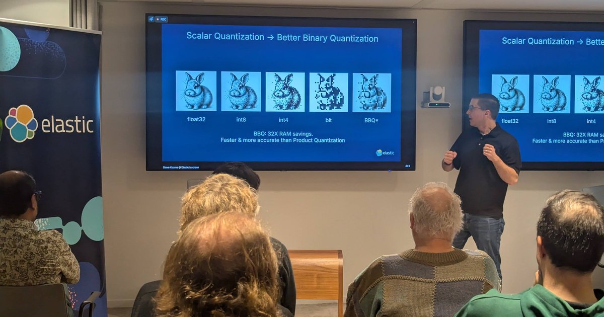
At the end of November 2024 I spent two days in a row with the Elastic community in Amsterdam. On Monday 25 November I went to the Elastic Meetup Amsterdam, the evening before ElasticON. It had three talks: Elastic on vector search, Kaufland on running e-commerce search, and Devoteam on observability for large Elastic Cloud Enterprise (ECE) platforms. On Tuesday 26 November I went to ElasticON Amsterdam at the Beurs van Berlage.

This post is a throwback built from the photos I took. I’ve only included what was on the slides and signs. At the end I add my own view on running quantized vector search in production.

Steve Kearns: the secret sauce of faster, better vector search

The first talk was by Steve Kearns, GM Search Solutions at Elastic according to his title slide. The talk was called “The Secret Sauce of Faster, Better Vector Search”. An early slide called Elasticsearch “the most widely deployed vector database”. That’s Elastic’s own claim. The talk then followed vector search through the 8.x releases.

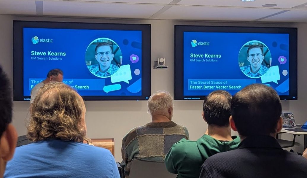
Steve Kearns’ title slide at Elastic Meetup Amsterdam, 25 November 2024.

int8 scalar quantization, on by default

The “Next Phase of Scalar Quantization” slide had three columns:

• Float32 to int8 in ingest. The slide gave the formula int8 ≈ 127 × (float32 − min) / (max − min) and listed lower cost, improved performance and “negligible ranking impact”.
• …on by default. About three quarters less index size and cost, better query latency, better ingest performance, and all of it “done within Elasticsearch (no effort)”.
• flat and int8_flat index types for small sets after a filter. When a filter leaves only a few documents, brute-force vector search works best. flat is “syntactic sugar for brute force”, and int8_flat adds automatic scalar quantization to it.

The next slide compared the trade-offs, using the same rabbit drawing at each precision. float32 keeps high recall and precision but needs all its vectors in RAM. int8 gives 4× RAM savings with good recall and moderate oversampling, and an arrow labelled it the “Elasticsearch 8.14+ default”. int4 gives 8× savings, but recall drops and oversampling becomes necessary. A single bit per dimension gives 32× savings with “bad” recall and precision.

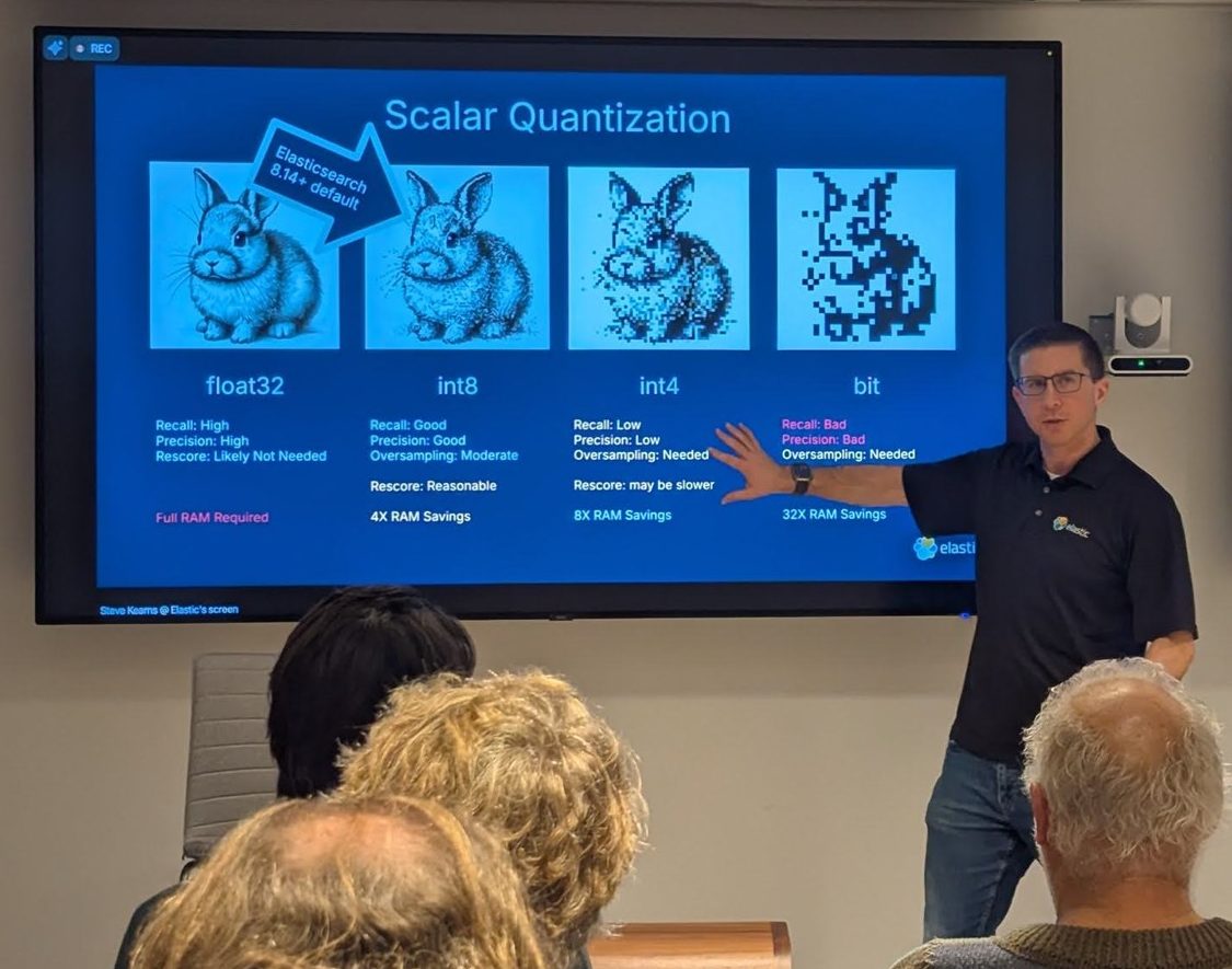
float32, int8, int4 and bit: recall, precision, oversampling and RAM savings, with int8 as the 8.14+ default.

Elastic’s documentation agrees. The Elasticsearch 8.14 release blog and the dense_vector field reference say that new dense_vector float fields use int8_hnsw by default from 8.14. Indices created on earlier versions keep plain hnsw.

Better Binary Quantization: 32× less RAM

Next came a slide titled “Good, but could it be better?” with a chart: memory in MB for 500k vectors of 1,024 dimensions. float32 needed 2,133.5 MB, int7 548.3, int4 292.3 and bit 66.7. The slide asked “100M vectors? Only 12GB!?!” and answered “Too good to be true!”

That set up Better Binary Quantization (BBQ). The slide said “BBQ: 32X RAM savings. Faster & more accurate than Product Quantization”. In the rabbit drawings, BBQ looked much closer to the original than plain bit did.

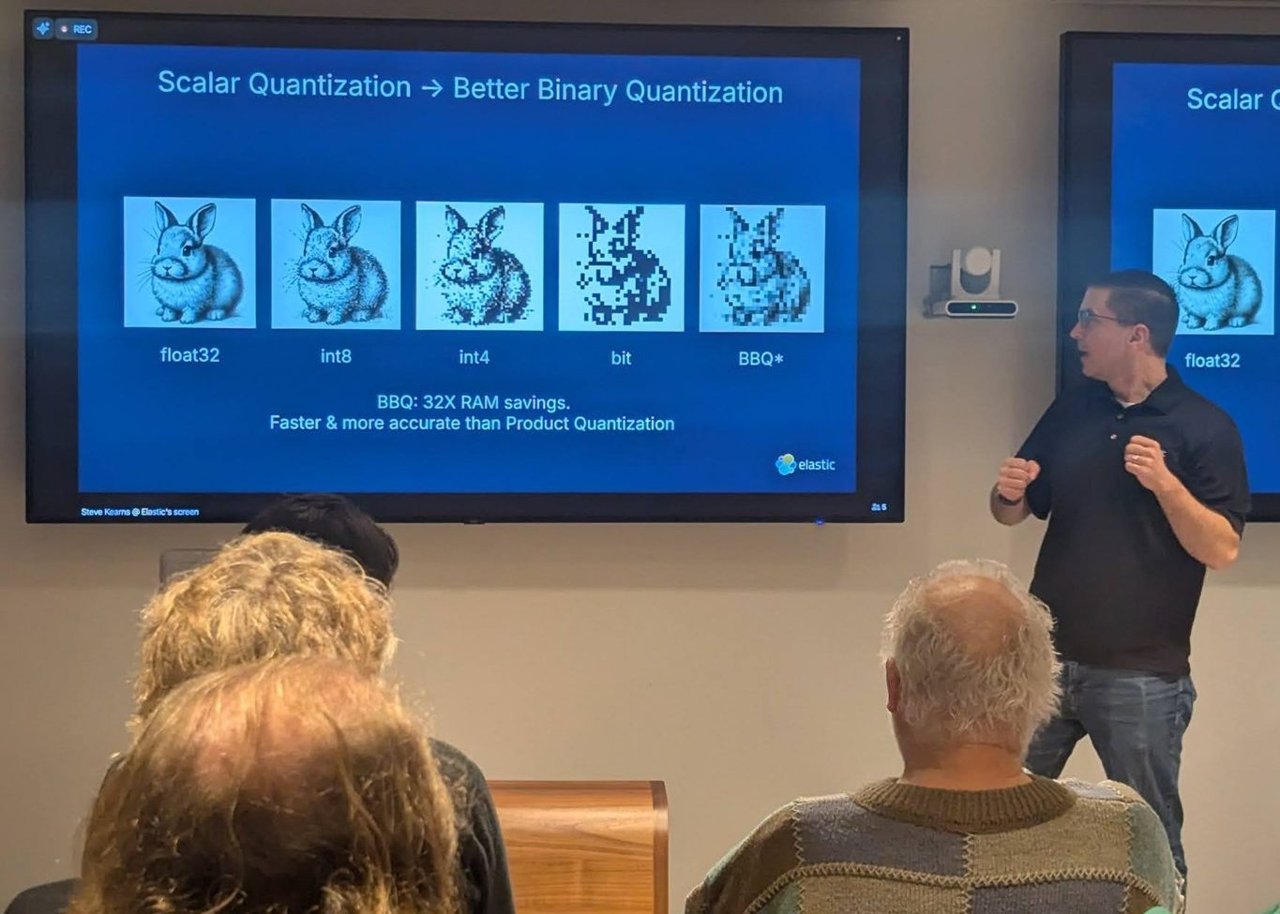
From scalar quantization to BBQ: 32× RAM savings, according to the slide.

The following slides asked the obvious questions in turn: “But, how long to index?”, “OK, but recall?” and “OK, but what about larger scale? Does it still work?”. The answers were benchmark charts on E5-Small and Cohere v3 embeddings. The summary slide, “More than a cool name”, compared BBQ with product quantization (PQ):

• CohereV3, 30M vectors. PQ took 13× longer to quantize than BBQ. Brute-force search at 98%+ recall was 3× slower with PQ.
• E5-Small, 500k vectors. PQ took 56× longer to quantize and searched about 2× slower.
• The two takeaways on the slide were “10–50x faster quantization speeds” and “2x or better query speeds”.

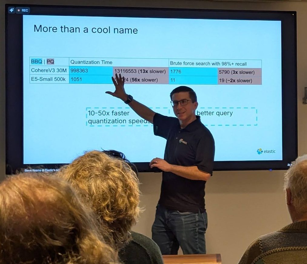
BBQ against product quantization: quantization time and brute-force search at 98%+ recall.

Elastic’s Elasticsearch 8.16 release blog, published on 12 November 2024, introduced BBQ, so the feature was about two weeks old at the time of the meetup. The blog describes up to 32× compression and “over 95%” less memory. The Search Labs post on BBQ in Lucene and Elasticsearch explains how it works: the stored vectors are single bits, the queries are quantized to int4, and the method builds on the RaBitQ research. Since then, the default has moved again. Elastic’s 9.1 post made BBQ the default quantization for dense vectors of 384 dimensions or more.

Hardware, retrievers and ES|QL

The “Hardware Optimization” slide covered three things:

• Panama-accelerated hardware instructions, with about 30% better query latency and indexing performance “if hardware supports it”.
• Fused multiply-add for dot products.
• A vector distance function optimised with SIMD: 3–6× faster, in native code, and for int8 on ARM AArch64 processors “under certain conditions”.

Then came retrievers and RRF, which the slide marked GA. The diagram had three stages. A standard semantic query and a knn query each return a result set. Reciprocal rank fusion (rrf) combines and ranks them. A text_similarity_reranker then reranks the combined list semantically. The example query was “why are retrievers fun?”.

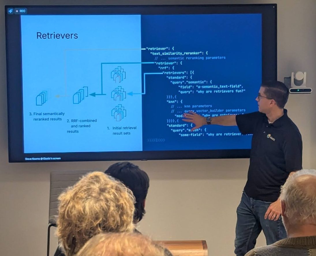
Retrievers: initial result sets, RRF fusion, then a semantic reranker, all in one request.

The talk ended with the ES|QL roadmap in three groups:

• Search, embeddings and RAG: full-text search, reranking, inference and multi-step querying.
• Time series, metrics and observability: time series data streams (TSDS) and a metrics command.
• Aggregations that keep the data: STATS and INLINESTATS.

Kaufland: e-commerce search and the road to Elasticsearch 8

The second talk came from Kaufland e-commerce. The opening slide described it as an online B2C marketplace with 11k sellers, more than 800 employees and five storefronts (de, cz, sk, pl, at). The speaker’s name wasn’t on the slides I photographed, so I won’t name them.

The architecture slide had three services: an Indexer, a Monolith and a Searcher. Around them were Kafka, BigQuery and Elasticsearch. The indexer reads from Kafka and BigQuery and writes to Elasticsearch, and the monolith and the searcher read from Elasticsearch.

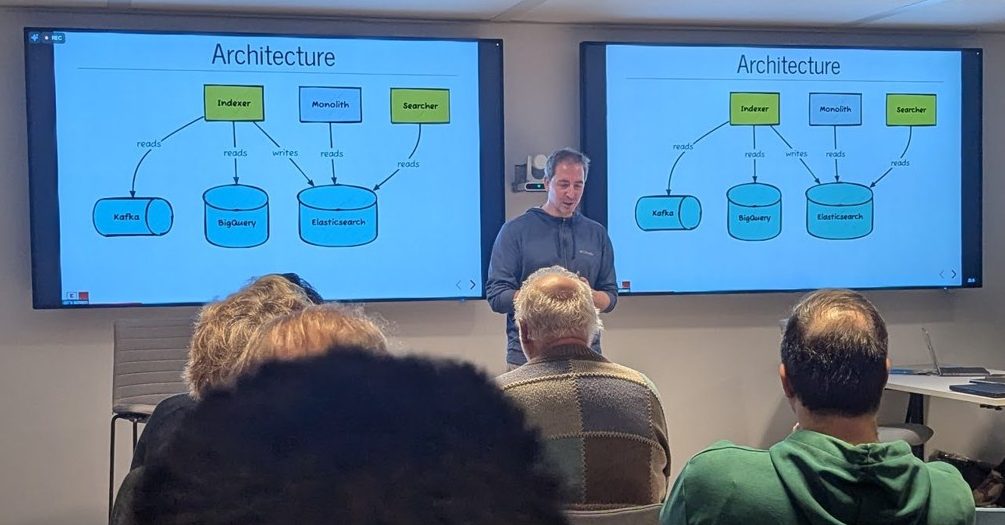
Kaufland’s search architecture: an indexer, a monolith and a searcher around Kafka, BigQuery and Elasticsearch.

The talk went through the phases of building relevance:

• Analysis. They used “search learner” data on how users interacted with search terms, and looked at shorter queries by asking “what are the important parts of this query?”.
• Search. A filter removes invalid products and handles shorter queries. A term-centric must query is multiplied with function_score, using field_value_factor for product rank and script_score for search learner rank.
• FTS vs. signals. The slide said the two are “tough to balance with a single query” and that signals are strong in the bigger storefronts. It also asked: “Do you really need FTS scoring, or just boolean matching?”

Then there was a quiz on minimum_should_match.

The second half was the journey to Elasticsearch 8. The timeline went from 7.12.1 in January to 7.17.22 in March and then 8.14.1 in May. On the way they hit:

• Node caches filling up, which pushed query latency up. A cron job to clean the caches worked around an unfixed bug in 7.17, but it introduced another bug that needed restarts.
• Unreleased shard locks. A disk ran full because other shards were being moved around, and the locked shards couldn’t be moved away. The fix was the 8.x upgrade.
• Less scripting. “Check if scripting is needed, if not: remove!”
• Unexpected refreshes. refresh_interval was set to 5m, yet there were dozens of refreshes within five minutes. The reason: the Update API calls a realtime GET, and when the translog location isn’t available, that GET triggers a refresh.
• Setting eager_global_ordinals, and a range query vs. term query difference that “seems to have been fixed in 8.x”.
• Tracking total hits. On a hot dataset with must/should/filter clauses and 11k results, track_total_hits: false took 400 ms and track_total_hits: true took 200 ms. The slide’s verdict was “WTF?”, and the explanation was dynamic pruning not working as expected with rank_feature.

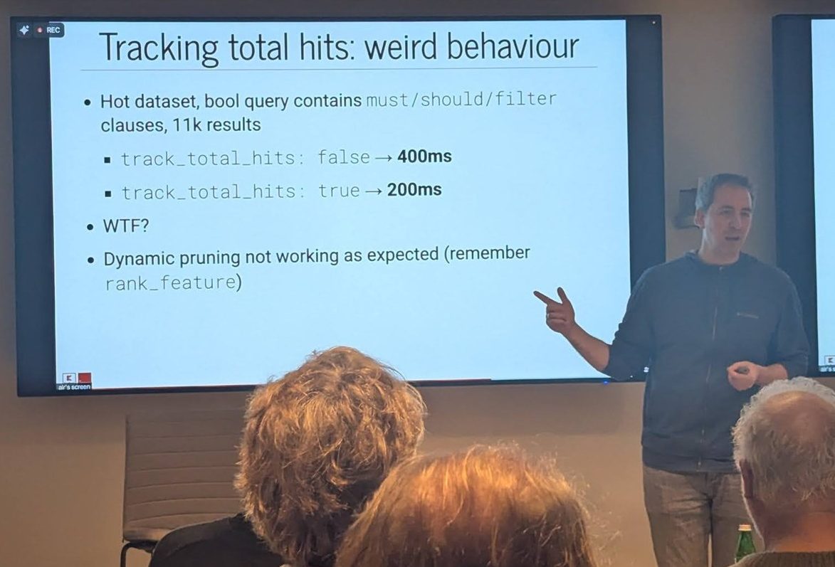
Turning track_total_hits off made this query twice as slow: dynamic pruning was not doing what they expected.

The last technical slides covered switching off a microservice to drop one gRPC network hop. They also showed a separate cluster upgraded from 7.9 to 7.17, after which there was “much less GC, CPU” and some nodes could be removed.

The ElasticON agenda the next day had a Community Track session called “From Keyword Search to Data Science: Search evolution at Kaufland e-commerce”, so the story continued there.

Devoteam: observability at scale with ECE

The third talk was “Observability at Scale — With ECE managed elasticsearch deployments” from Devoteam. Patrick Broek, Lead Consultant, presented the observability part. The title slide listed a second Devoteam consultant as co-presenter, and a second presenter took over for the automation part.

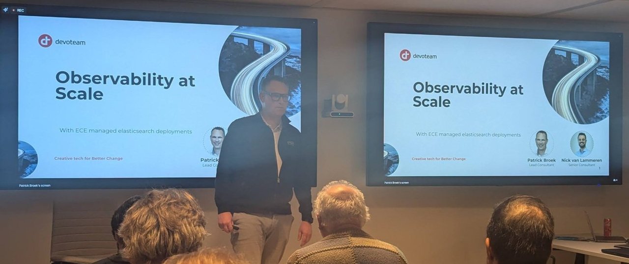
Devoteam’s “Observability at Scale” with ECE-managed Elasticsearch deployments.

The talk started with the ECE high-level architecture. The control plane holds the Cloud UI, the Admin API, ZooKeeper plus the Director, and the Constructor. Proxies sit behind a user-supplied load balancer, and allocators run the deployments, with separate ES Admin and ES Logging clusters. Next came a platform summary of capacity and role distribution across zones, and the question “How do you build observability on ECE?”. The answer combined the ECE platform APIs (/api/v1/platform/infrastructure/allocators and /api/v1/deployments) with GET _nodes/stats filtered to data-set size, roles and names. The result was a view of allocators per tier and zone.

The “What can we gain from this” slide listed:

• insight into hundreds of deployments plus ECE itself
• alerting at the right level
• lifecycle management
• capacity planning
• KPI dashboards and reporting
• “much more”: unassigned shards, Logstash error monitoring and infrastructure patch monitoring

The automation section listed three key requirements: scalable, centralised control with low effort, and source code management. The tools slide shows how they put it together: Ansible in the middle, connected to Terraform, PostgreSQL and git, with Terraform pointing at Elastic and Budibase on top of PostgreSQL.

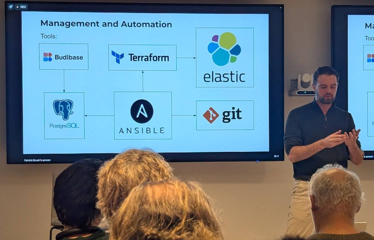
Management and Automation: Ansible at the centre, with Terraform, PostgreSQL, git, Budibase and Elastic around it.

My take: this is the right shape for a large ECE estate, with Ansible and Terraform rather than clicks in a UI. When you have hundreds of deployments, the platform only stays manageable if its state lives in git and a tool applies it.

ElasticON Amsterdam at the Beurs van Berlage

The next day ElasticON took over the Beurs van Berlage. According to the agenda board, the day ran from 07:30 to 18:45 in the Grote Zaal, Effectenbeurszaal, Administratiezaal and Beursfoyer. Some of the sessions on the board:

• the welcome keynote, “Supercharge <anything> with Search AI”
• a customer keynote from Volvo Cars
• “Build trusted, production-ready generative AI applications on Elasticsearch”
• “Exploring Re-Ranking Techniques for E-commerce Search”
• “The Future of Elasticsearch Queries: Exploring ES|QL and What’s Next”
• the Kaufland session mentioned above

The lunch break had lightning talks: “Actioning AI: Elastic Insights with Tines Workbench”, “Hybrid Geospatial RAG with Elastic and Amazon Bedrock”, and an ElastiFlow lightning talk.

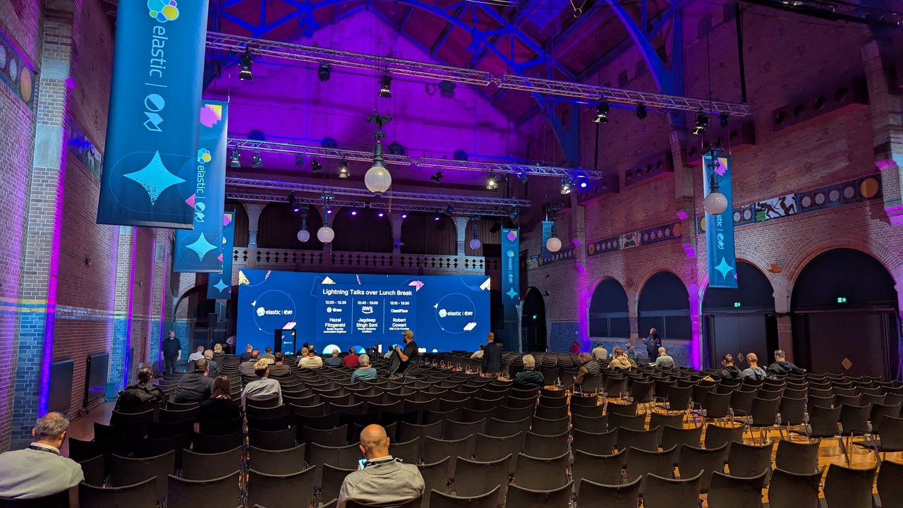
Lightning Talks over Lunch Break at ElasticON Amsterdam, in one of the Beurs van Berlage halls.

In the expo area there was a Customer Advocacy corner in the Elastic Acceleration Zone, which promised an ELK(Y) plushie to the first 50 customers who completed a review. There were also screens for the Elastic Excellence Awards. The sponsor wall thanked AWS, Tines, ElastiFlow and Kangaroot, among others.

Me at the ElasticON sponsor wall.

My take: quantized vector search in production

My take: the most useful thing about this meetup was that it treated quantization as a capacity-planning lever, not a research topic. Quantization is now on by default: int8 since 8.14, and BBQ for 384+ dimensions since 9.1. So many teams already run quantized vectors without ever having chosen to. That’s fine, as long as you know it and measure it.

What I’d do on a production cluster:

• Measure recall on your own queries, not just on public benchmarks. Keep a small labelled set from real traffic and compare float32 against the quantized index before and after every mapping change.
• Tune oversampling and rescoring on purpose. The trade-off slide said it plainly: lower precision needs more oversampling. The dense_vector docs expose this as rescore_vector.oversample. Treat it like any other latency/quality knob and track it in your dashboards.
• Plan RAM and disk separately. The RAM savings are real: the slide’s 500k × 1,024 example went from about 2.1 GB to under 70 MB with bits. If you rescore, though, you still keep the full float vectors on disk.
• Use flat or int8_flat where filters already shrink the candidate set. Kearns’ slide made that point, and it applies directly to multi-tenant search: when a tenant filter leaves only a few thousand documents, an HNSW graph isn’t worth it.
• Upgrade, then re-index. According to the docs, the defaults depend on the version an index was created on. Upgrading the cluster, as Kaufland did on its way to 8.14.1, doesn’t change the quantization of an existing index.

Related

• ElasticON Amsterdam 2025: Forge the Future Recap
• AI Native Netherlands at Elastic: Agents, MCP, Workflows
• Elastic Agent Builder MCP: Tools and Workflows, No LLM
• SRE NL at Elastic: OpenTelemetry and Your Brain’s Biases
• Vector Databases on Kubernetes: Qdrant vs Milvus vs pgvector
• Loki vs Elasticsearch 2026: Log Aggregation Comparison